COMSOL

Finite Element Analysis (FEA) is a computational method used in microfluidics and electrokinetic biosensor research to analyze and simulate the behavior of fluids, electric fields, and particles at the microscale level. It involves dividing complex geometries into smaller, finite elements, allowing for accurate modeling and prediction of fluid flow, electrokinetic phenomena, and particle transport within microfluidic devices and electrokinetic biosensors.

In microfluidics, FEA helps in understanding fluid behavior, such as pressure distribution, velocity profiles, and mixing efficiency, within intricate channel networks. It enables researchers to optimize device designs, predict flow patterns, and evaluate the performance of various microfluidic components, such as valves, pumps, and mixers. FEA also aids in studying phenomena like droplet formation, particle trapping, and droplet merging, providing insights for the development of advanced lab-on-a-chip systems.

Regarding electrokinetic biosensors, FEA assists in simulating electric fields, ion concentration distributions, and the movement of charged particles within microchannels. It enables the analysis of electroosmotic flow, electrophoresis, dielectrophoresis, and other electrokinetic phenomena relevant to biosensing applications. By utilizing FEA, researchers can optimize electrode geometries, electrode configurations, and operational parameters to enhance the sensitivity, selectivity, and overall performance of electrokinetic biosensors.

Analysis of fluid performance of micromixer with and without obstacles inside of microchannel

In the field of mechanics, a micromixer is a device that utilizes mechanical microparts to mix fluids. This technology holds significant importance in various industries, such as the chemical and pharmaceutical sectors, analytical chemistry, biochemical analysis, and high-throughput synthesis. The micromixer takes advantage of fluid miniaturization to reduce the quantities involved in chemical and/or biochemical processes, making it a key tool in these applications.

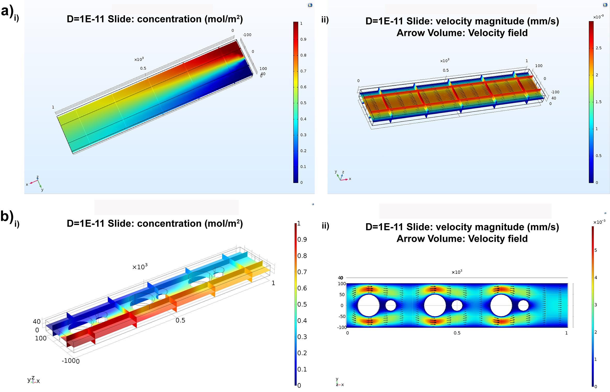
In the passive micromixer, obstacles were strategically positioned inside the microchannel to interrupt the flow and minimize the diffusion path. This disruption of the flow velocity field causes the flow direction to interact with another fluid, resulting in convection that significantly enhances the mixing process. Model 1 was designed as three-dimensional rectangle straight channel with 1000 µm* 200 µm* 50 µm in Width, Length and Hight. Model 2 was designed based on model 1 but incorporated six circle-shaped obstacles symmetrically placed at the center of the channel. A comparison with a straight channel revealed that the mixing efficiency was significantly improved, even with species possessing the same diffusion coefficient. Fig. b demonstrates that the two fluid flows required a longer distance to achieve uniform mixing. Notably, the simulation results revealed fluid velocity constrictions around the circular obstacles, highlighted in red color. These constrictions arose as the fluid encountered the obstacles, resulting in the highest speeds. In this well-designed configuration, the two fluid flows from separate inlets were skillfully diverted to the sides of the channel, effectively preventing the diffusion of the two species as they encountered the obstacles.

Concentration and velocity profiles of two passive micromixers: without/with obstacles;

Electroosmotic micromixer

Electroosmotic flow arises from the electric field acting on the electrical double layer at the fluid/solid interface, which is determined by the surface charge of the solid surface. The flow inside the channel is mathematically described by the Navier-Stokes equation. A frequently encountered simplification in electroosmotic flow analysis is the “Helmholtz-Smoluchowski” approximation, which relates the electroosmotic velocity to the tangential component of the applied electric field.

In the model one, a straight channel in nano-size with non-uniform charged surface was developed to mix fluids under electric field as 0.006 V applied at the inlet and the outlet of the channel. Electroosmotic flow in the channel was determined by Navier-Stokes equation in the approximation of the creeping flow. In addition, the no slip boundary condition was used at the solid interface. The channel surface was divided into three parts and carried an estimate surface charge (sigma) as -0.02 C/m2 and 0.06 C/m^2. The second model, the electroosmotic micromixer took two fluids from different inlets and combine them into a single channel which is 10 µm wide. The fluids entered the central loop with 5 µm and 15 µm respectively. Four microelectrodes are positioned on the outer wall of the loop at the angular position 45°, 135°, 225°and 315°. The fluids inside of the loop were manipulated through the electroosmotic slip boundary condition. Also, electric potential applied on the electrodes were time-dependent. Over two entire models, the initial condition for constant temperature was assumed to be 300 K and pressure as 0 Pa.

Concentration and velocity profiles of electroosmotic micromixers

Analysis of fluid flow in Nanopore sensing

Finite Element Analysis (FEA) presents significant benefits in nanopore biosensor design and optimization. It involves dividing complex structures like nanopores into smaller, manageable elements to simulate their behavior under different conditions. In nanopore biosensor development, FEA provides crucial insights into fluid flow patterns, electric field distribution, and molecular interactions within the nanopore system.

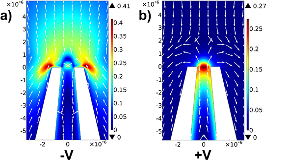
The fluid flow and electric field inside a 1 μm inner diameter micropipette, suspended in a reservoir of 1 mM KCl solution were simulated. The nanopore was represented with a conical protrusion extending to the pore tip, focusing on the near-pore region to study flow physics under applied bias. The pipette’s wall had inner and outer taper angles set to 5 degrees and 13 degrees, respectively. The reservoir, mimicking the actual experimental environment, had a circular shape and was designed large enough to approximate infinity. It was modeled with permittivity values of 4.2 and 80 for glass and water, respectively. The glass surface carried an estimated surface charge of 0.02 C m^-2. Throughout the model, the initial conditions were set with a constant temperature of 298 K, zero pressure (0 Pa), and an initial voltage bias of zero volts. However, a DC bias of 30 V was applied at the base using a 2 nm wide electrode region, simulating a voltage source. Figures below represent the fluid flow pattern of near tip region up to 6 μm distance from the pore. The size of the arrows is proportional to the magnitude of fluid velocity and is evidently larger near the pore compared to the bulk solution.

Fluid flow pattern for a 1 μm diameter pore in the near tip region with applied a -30V and b +30 V at the base in 1 mM KCl solution

Analysis of electric field distribution in electrochemical impedance spectroscopy (EIS) sensing platform

Analyzing the electric field distribution in an electrochemical impedance spectroscopy (EIS) sensing platform offers several key advantages. EIS is a powerful technique used to study the electrical properties of electrochemical systems. By analyzing the electric field distribution, we can gain insights into the interactions between analytes and electrodes. Understanding the spatial distribution of the electric field provides valuable information about the kinetics and mechanisms of the electrochemical processes occurring at the electrode surface. This knowledge is crucial for optimizing sensor performance and sensitivity. Additionally, studying the electric field distribution helps in the design and modification of electrodes to enhance the sensor’s detection capabilities.

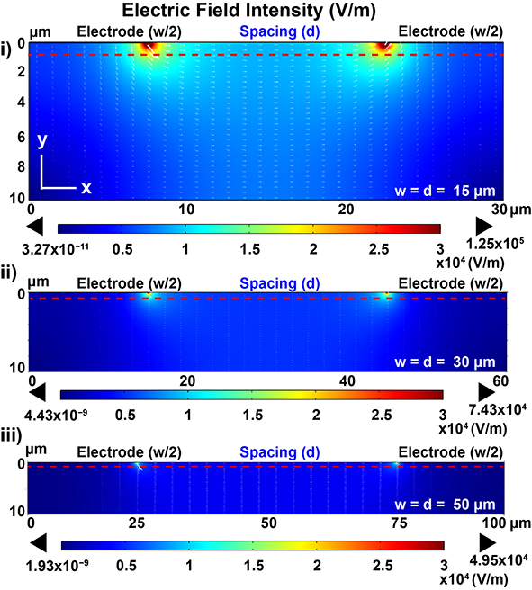
The simulated 2-D cross-section included an interdigitated electrode on the glass substrate and the ambient fluid (0.1 × PBS solution). To reduce complexity, the model included only two fingers of the replicating electrode structure with opposite voltage polarity [34,44] (Figure 4a). The dimensions of the electrode were defined as width (w = 15 μm, 30 μm, and 50 μm), spacing (d = 15 μm, 30 μm, and 50 μm), and height (h = 100 nm). Current conservation was applied to the whole domain, and the outer boundaries were adopted as electric insulation. Voltage terminals were applied to the electrodes (−100 mV and 100 mV), respectively. The electrodes were meshed with 0.003 μm as the minimum element size and 0.2 μm as the maximum element size, and the maximum element growth rate was specified to be 1.3.

Figure below shows the electric field intensity near the electrode region (10 μm below the electrode surface), where the binding between the cells and immobilized antibodies is expected. The simulation demonstrated that the highest electric field was confined at the edge of the electrodes and decayed along the y-axis. The electric field intensity at smaller electrode dimensions (peak intensity: 12.5 kV/m for 15 μm) was found to be higher than the larger dimensions (peak intensity: 7.43 kV/m for 30 μm; 4.95 kV/m for 50 μm).

2D cross-section simulation of electric field distribution of IDEs at (i) 15 μm; (ii) 30 μm; (iii) 50 μm;